The Linear Model

Welcome!

This is a short refresher of the linear model and Ordinary Least Squares by SuffolkEcon, the Department of Economics at Suffolk University. It covers the basics of parameter estimation and inference. It does not cover model diagnostics.

Comments? Bugs? Drop us a line!

To go back to the SuffolkEcon website click here.

Preliminaries

If you are new to R, we recommend you do the following tutorials before this one:

Set-up

Packages

We’ll use the tidyverse and SuffolkEcon. Invoke them the usual way by typing library(tidyverse) and library(SuffolkEcon) in the chunk below:

library(tidyverse)
library(SuffolkEcon)

Data

We’ll use the data set hprice (from the SuffolkEcon package) to study the relationship between house prices (the column price) and clean air (the column nox or Nitrogen Oxide, a pollutant).

data("hprice", package = "SuffolkEcon")
hprice

What is a model?

Abstractions

A model is an abstraction. It strips away certain details to focus on the essence of something. Like a paper airplane, or Picasso’s famous bull lithographs:

‘The Bull’ (1945) by Picasso

In econometrics we use models to study relationships between variables, like house prices and air pollution.

Linear Abstractions

The linear model is an abstraction that imagines the relationship between two variables as constant. A constant relationship can modeled with a line.

For instance, we might expect that the price of house ($\text{Price}$) is a function of air pollution ($\text{NOX}$, Nitrogen Oxide):

\[ \text{Price}= f(\text{NOX}) \]

where $f(\cdot)$ is some function.

In the linear model, that function $f(\cdot)$ is a line:

\[ \begin{aligned} \text{Price} &= f(\text{NOX}) \\ &= \beta_0 + \beta_1\text{NOX} \end{aligned} \] where $\beta_0$ is the intercept of the line, and $\beta_1$ is the slope of the line.

The slope is what captures the relationship between prices and pollution.

For instance, if we think there is a negative relationship (more pollution, lower prices), our model would like something like this:

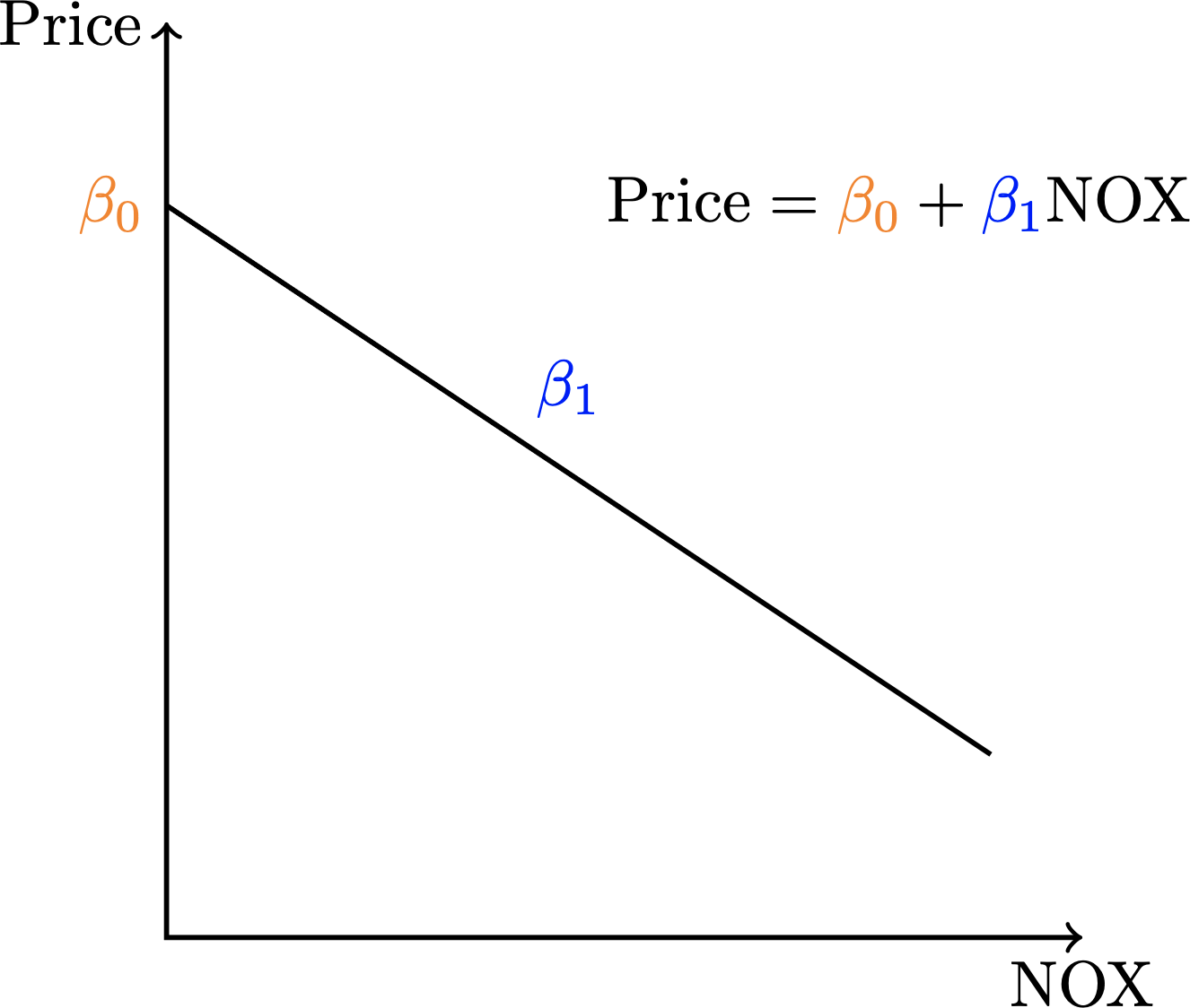
A negative and linear relationship between pollution and house prices

Prices and Pollution

Make a scatter plot of price (price, thousands of dollars) against pollution (nox, parts per million).

Recall the general format of a scatterplot, where data is the name of your data set, and x_variable and y_variable are columns in the data set:

data %>% # data, THEN
  ggplot(aes(x=x_variable, y=y_variable)) + # blank canvas with axes
  geom_point() # scatterplot layer

hprice %>% 
  ggplot(aes(x=nox, y=price)) + 
  geom_point()

It looks like there is a negative relationship: more pollution, lower prices.

We can model this relationship with a line by adding a linear regression to the plot. Re-do the plot, but this time add (+) geom_smooth(method = 'lm'):

data %>% # data, THEN
  ggplot(aes(x=x_variable, y=y_variable)) + # blank canvas with axes
  geom_point() + # scatterplot layer 
  geom_smooth(method = 'lm')

hprice %>% 
  ggplot(aes(x=nox, y=price)) + 
  geom_point() + 
  geom_smooth(method = 'lm')

Estimating parameters

Linear regression: the algorithm

Linear regression uses an algorithm called “Ordinary Least Squares” (OLS) to estimate the parameters of a model.

It’s a pretty simple algorithm: it takes a spray of points and draws a line through them.

But how does it choose the line? By minimizing error. More specifically, by minimizing squared error.

Error is the difference an observed data point and the predicted data point from the model. In the GIF below error is the difference between the line (prediction) and the points (data):

Least Squares (credit to https://bit.ly/3ynRnog)

OLS squares the errors so negative and positive errors are comparable. Hence “least squares”.

Models and parameters

Our linear model is

\[ \begin{aligned} \text{Price} &= f(\text{NOX}) \\ &= \beta_0 + \beta_1\text{NOX} \end{aligned} \]

$\beta_0$ and $\beta_1$ are the parameters of the model – the values we want to estimate.

We are most interested in $\beta_1$ – the slope of the blue line in the plot. It tells us how prices change as pollution changes.

Of course, we know that house prices are affected by other stuff besides pollution. We have some other variables in our data set, but they probably do not cover all the factors that affect prices. There is some randomness that we can account for by adding an error term to our model:

\[ \begin{aligned} \text{Price} &= f(\text{NOX}) \\ &= \beta_0 + \beta_1\text{NOX} + \varepsilon \end{aligned} \]

where $\beta_1$ is the effect of pollution on prices and $\varepsilon$ captures the effect of everything else on prices.

`lm()`

Use the function lm() to estimate the parameters of a linear model:

lm(formula = y ~ x, data = data)

where y is price, x is nox and data is hprice:

lm(formula = price ~ nox, data = hprice)

Interpretation

In the linear model, $\hat{\beta_1}$ (“beta one hat”) is interpreted this way:

A one unit increase in $x$ is associated with a $\hat{\beta_1}$ change in $y$, on average.

So, according to our results, an increase in one parts per million of Nitrogen Oxide is associated with an average decrease of -$3,387.00 in house prices.

Randomness and Order

So we estimated $\hat{\beta_1} = -3387$.

But how stable is this estimate?

Regression coefficients are random variables

If we draw a new sample of houses, we will probably estimate a different pollution effect.

See this for yourself by running the chunk below several times. It’s an experiment: it pretends the data hprice is a population, draws thirty random houses, and re-estimates the model:

hprice %>% # take the data, THEN
  slice_sample(n=30) %>% # draw a random sample of 30 houses, THEN
  lm(formula = price ~ nox, data = .) # estimate the parameters of the linear model

Notice how the coefficient on nox changes each time!

Random variables have distributions

The good news is that random variables have structure in the form of distributions – shapes that tell you which outcomes are most likely.

If we were to run this experiment many times and plot the distribution of coefficients – the sampling distribution – it will be structured like a bell-shaped normal distribution.

It’s like saying, “what if we ran the experiment many times? What would be the average estimate?”

Let’s do this with the function what_if(). First we’ll run 10 experiments:

hprice %>% 
  SuffolkEcon::what_if(model = price ~ nox, experiments = 10, sample_size = 30)

and then we’ll run 1000 experiments:

hprice %>% 
  SuffolkEcon::what_if(model = price ~ nox, experiments = 1000, sample_size = 30)

and we can see the that the distribution of coefficients becomes more normal with more experiments, and that average or center of this distribution is close to our original estimate of -3300.

Inference

We just saw that regression coefficients are random variables that vary across samples.

We also saw that running an experiment – draw sample, run regression – many times produces a sampling distribution that becomes more normally distributed with more experiments.

So how do we know if the center of that distribution is meaningful – different from zero?

Because if the true value of $\beta_1$ were zero, then pollution would have no effect on prices:

\[ \begin{aligned} \text{Price} &= f(\text{NOX}) \\ &= \beta_0 + \beta_1\text{NOX} + \varepsilon \\ &= \beta_0 + (\beta_1=0)\text{NOX} + \varepsilon \\ &= \beta_0 + \varepsilon \end{aligned} \]

So, we use our sample hprice to infer – to see if the relationship in our sample would hold for any sample drawn from the population.

Hypothesis testing

Inference starts with a hypothesis. Is there or is there not an effect of pollution on prices?

We write this as

\[ \begin{aligned} H_0 &: \beta_1 = 0 \\ H_A &: \beta_1 \neq 0 \end{aligned} \]

The null ($H_0$) states the coefficient – the average of the sampling distribution – is zero. It is like saying “on average we should find no relationship between pollution and price”.

You can think of this in terms of the legal presumption of innocence:

\[ \begin{aligned} H_0 &: \text{innocent} \\ H_A &: \text{guilty} \end{aligned} \]

The idea is that the prosecutor (the researcher) must gather evidence (data) to reject the defendant’s innocence (i.e. reject $H_0$). If the data are lacking then you fail to reject the null hypothesis.

P-values

Innocent or guilty, fail to reject or reject

We cannot prove things with data.

Why?

Because we observe samples of the population, not the population itself.

We use those samples to infer about the population.

We then use hypotheses to do inference.

And since we cannot prove anything, we can only reject or fail to reject hypotheses.

Truth is a probability

How do we decide whether to reject or fail to reject? Using a probability called the p-value.

The p-value is the probability of observing $\hat{\beta}$, the estimated effect – assuming the null hypothesis (no effect; “innocent”) is true.

If the probability is very close to zero, then it is unlikely the null hypothesis is true, and we can reject it.

But if the probability is very close to one, the it is likely the null hypothesis is true, and we fail to reject it.

`summary()`

p-values are calculated for you with the function summary().

summary() takes the output of lm() and spits out the estimated coefficients, as well the hypothesis tests and other regression diagnostics.

The general format is

lm(formula = y ~ x, data = data) %>% # estimate the parameters, THEN
  summary() # conduct the hypothesis tests

where y is price, x is nox and data is hprice:

lm(formula = price ~ nox, data = hprice) %>% 
  summary()

Each row of the table corresponds to a coefficient.

Under the column “Estimate” we see the estimate for nox, same as before (about -3387).

The p-values are shown in the column Pr(>|t|).

Interpreting p-values

If the probability is very close to zero, then it is unlikely the null hypothesis is true, and we can reject it.

How close to zero is close enough?

There is no hard-and-fast rule. So science has coordinated on a set of thresholds so that the convention is to compare your p-values to some fixed thresholds like:

10% or 0.10: “weak evidence to reject $H_0$”
5% or 0.05: “evidence to reject $H_0$”
1% or 0.01: “strong evidence to reject $H_0$”

These thresholds are the false positive rates we are willing to tolerate (i.e., the rate at which we falsely conclude the effect is significant, if we were to repeatedly sample and test). If the p-value is below a threshold, say 5%, we say that we reject the null hypothesis at the 5% level.

And if we reject the null, we say the effect is statistically significant.

Since the p-value on nox is 2e-16 (a two with 16 decimals in front of it), it is below every coordinated threshold, and is therefore statistically significant.

Notice the “stars” (*) next to the p-value and “significance codes”:

Signif. codes:  0 '***' 0.001 '**' 0.01 '*' 0.05 '.' 0.1 ' ' 1

So three stars (***) means you can reject at the .1% level, two stars at the 1% level, and so on.

Illustrating p-values

The p-value is the probability of the test statistic under a true null hypothesis. Let’s unpack this.

The test statistic or t-value is the coefficient divided by it’s standard error. The test statistic for our coefficient on nox is -10.57:

-3386.9 / 320.4

and the p-value is simply the area underneath the curve of the t-distribution, which is centered at zero (the null hypothesis):

SuffolkEcon::plot_t_value(t_value = -10.57085, dof = 504)

It’s hard to see because the area is so small. If the t-value were smaller – closer to zero – the probability would be higher:

SuffolkEcon::plot_t_value(t_value = -1.0, dof = 504)

Much ado about p-values

Sometimg to keep in mind about p-values is they are massively influenced by the amount of data. This is because the test statistic is the coefficient divided by the standard error, and the standard error is divided by the square root of the number of observations.

For instance, if we run 100 experiments and drew only 10 observations each experiment, we won’t always reject the null hypothesis on nox:

hprice %>% 
  SuffolkEcon::what_if(model = price ~ nox, experiments = 100, sample_size = 10, p.values = TRUE)

and it makes no difference if we run more experiments:

hprice %>% 
  SuffolkEcon::what_if(model = price ~ nox, experiments = 1000, sample_size = 10, p.values = TRUE)

But the rejection rate goes way up when we increase our sample size:

hprice %>% 
  SuffolkEcon::what_if(model = price ~ nox, experiments = 100, sample_size = 100, p.values = TRUE)

Multiple regression

Pollution is probably not the only thing that influences a home buyer.

They might also care about crime (the column crime), property taxes (proptax), and school quality (stratio, the student-teacher ratio).

If we don’t account for these factors, then our model suffers from omitted variable bias.

We turn our simple regression into a multiple regression by simply adding these variables.

The general framework is:

lm(formula = y ~ x1 + x2 + x3, data = data)

Try adding crime and proptax to the model and use summary() to view the coefficients and hypothesis tests:

lm(formula = price ~ nox + crime + stratio, data = hprice) %>% 
  summary()

Notice that the coefficient on nox is still negative and significant, meaning there is likely a negative relationship between pollution and prices. At the same time, the coefficient is smaller in our new model, because in the first model we did not account for the effects of crime and school quality.

Working with `lm` objects

One last note. lm() returns an object. You can view objects with the class() function:

lm(formula = price ~ nox, data = hprice) %>% 
  class()

In R you can store anything in an object. So you can store the output of lm() into your own object, like estimated_parameters, and then pass that object to summary():

# estimate the parameters and store them
estimated_parameters = lm(formula = price ~ nox, data = hprice)
# run the hypothesis tests on the estimated parameters
summary(estimated_parameters)

Notice the output is the same as when we did

lm(formula = price ~ nox, data = hprice) %>% 
  summary()

Saving the output of lm into an object is useful because you can then plot the estimated coefficients or marginal effects using the sjPlot package, or print a table (Word, PDF or HTML) using the stargazer package.

Check out the resources page to learn about other packages that work with regression objects.