Welcome!
This is a short introduction to R programming by SuffolkEcon, the Department of Economics at Suffolk University.
Comments? Bugs? Drop us a line!
To go back to the SuffolkEcon website click here.
What will you learn in this tutorial?
Some fundamentals of R.
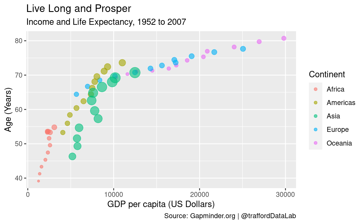
At the end we will look at data on income and life expectancy and recreate this plot:

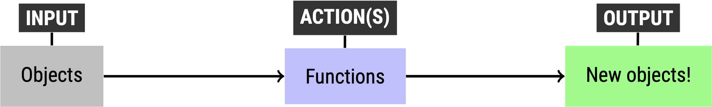
The big idea
Say you want to make an omelette. It goes something like this:
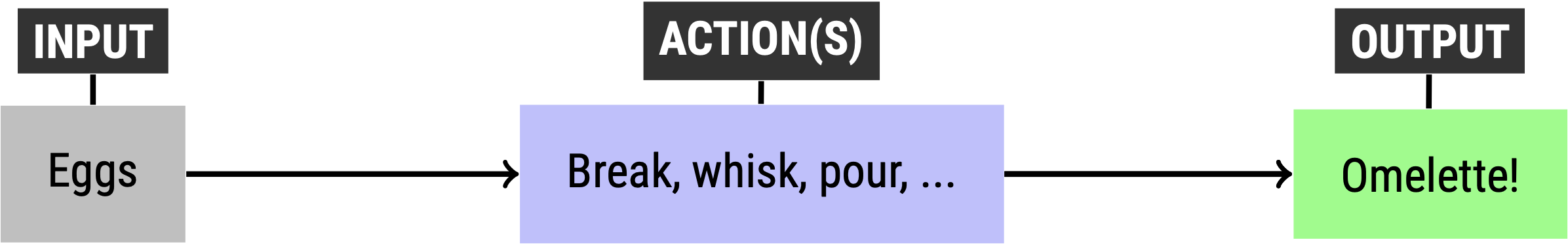
Programming in R follows the same basic input \(\rightarrow\) action \(\rightarrow\) output framework:
Keep this framework in mind as you work through the tutorial.
R the Calculator
The simplest way to use R is as a calculator.
For example, the code below calculates \(1+1\). Click the “Run Code” button in the chunk below:
1+1 # add one and oneand this code calculates \(2^3 + 4*5 + \frac{5}{6}\):
2^3 + 4*5 + 5/6 # two to the third plus four to the fifth plus five divided by sixExercises
Now you try. Calculate \(2^2 \times 3^3\):
2^2 * 3^3Comments
Do you remember what you had for breakfast last Tuesday? Probably not. Same goes for coding.
You will look back at code you wrote last week and realize you don’t what it does, or why you wrote it.
Comments are notes you write in the code to help you (or somebody else) understand what’s going on.
Let’s look at that first chunk we ran:
1 + 1 # add 1 and 1 The code spits out “2”, not “# add 1 and 1.” That’s because “#” is a comment. And everything after a “#” is ignored by R.
So: comment!
Commenting is important – especially when you are starting out.
What should you comment? Everything.
When should you comment? Always.
Why should you comment? Because you want to be nice to future self.
Objects: R’s Memory
x = 1 + 1 OK, we can use R to make calculations.
But what if we want to save the output of one calculation and use it in another calculation?
R has memory. What does it remember? Whatever you tell it to! This is called defining objects.
Defining objects
An object can be many things. Let’s try a simple one.
Suppose we want to calculate \(1+1\) and store it in an object. We have to give it a name. Let’s call it “x”. Run this code:
x = 1 + 1 # add 1 and 1, then assign the output to "x"Notice two things:
=is the assignment operator. It says: "take 1+1 and assign its output tox.- When we run the code,
x = 1 + 1, nothing spits out. That’s because the output is stored inx.
Let’s see what’s inside x by printing it. We should this code spit out “2”:
x # print "x" to the screenIt worked!
R will now remember x. That means we can use x in another calculation.
For example, let’s calculate \(x+1\):
x + 1 # add 1 to each element of xWe can do math with multiple objects. Let’s define an object x2 equal to 2 and then calculate \(x + x_2\):
x2 = 2 # assign the number 2 to the object "x2"
x + x2 # add x and x2
Finally, you can rewrite R’s memory. For example, let’s redefine x:
x = 2 + 2 # redefine "x" as the output of 2 + 2
x # print the new x to the screen
Exercises
- Define an object called
y, assign \(2^2\) to it, and then printy:
y = 2^2
y- Now define an object called
z, assign \(y/2\) to it, and then printz:
y = 2^2z = y/2
zObjects: Vectors
x = c(5,10,15,20)So far so good. But science is about learning from many data points. So we need objects that can store many data points. The simplest are vectors.
Consider the vector \(\vec{x} = [5,10,15,20]\). To tell R to create this vector, we use the command c():
x = c(5,10,15,20) # create the vector [5,10,15,20] and assign it to "x"
x # print x to the screen
Once again we can do math with objects. Let’s calculate the mean of x:
mean(x) # calculate the mean of xOr let’s multiply each element of x by 2:
x*2 # multiply each element of x by 2Subsetting
We can work with all of x. Or we can work with one or a few elements of it. That’s because every element in \(\vec{x}\) (and x) has a numeric position:
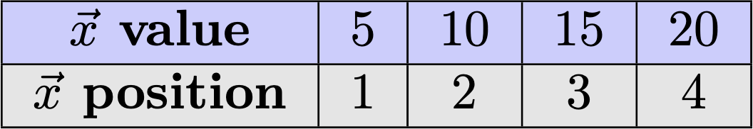
To slice a vector we use x[position].
For example, let’s look at the first element of x:
x[1] # show the first element of xor let’s take the third element of x – 15 – and add three:
x[3] + 3 # take the third element of x and add threeExercises
- On line 1, create a vector \(\vec{y} = [1,2,3,4]\). Then on line 2, divide each element by four.
y = c(1,2,3,4)y = c(1,2,3,4)
y/4- On line 1, create a vector \(\vec{z} = [2,4,3,8]\). Then on line 2, use subsetting to multiply the last element of
zby the second element ofy.
z = c(2,3,4,8)
z[4]*y[2]
Objects: Data Frames
x = c(1,2,3,4,5) # create the vector x
y = c(6,7,8,9,10) # create the vector y
df = data.frame(x,y) # join x and y into a dataframe called "df"
You’ve probably seen an Excel spreadsheet before. Something like this table below. It has columns, each column has a header, and each header has data below it:
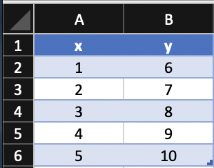
In R this is called a dataframe. And a dataframe is just an object that chains vectors together.
Creating a dataframe
Let’s create two vectors \(\vec{x}\) and \(\vec{y}\). Run this chunk to create them (nothing will get spit out, since we assigned the outputs to x and y):
x = c(1,2,3,4,5) # create a vector x
y = c(6,7,8,9,10) # create a vector y
We can combine them with data.frame(). As usual, we have to give our object a name. Let’s call it “df” for “dataframe”:
df = data.frame(x,y) # join x and y in a dataframe
df # print the dataframe to the screen
We see a column called “x” (that’s x), a column called “y” (that’s y), and on the left we see the number of rows. So df is a 5 (row) by 2 (column) data frame.
Subsetting
Just like you can subset vectors, you can access specific columns in data frames.
To access a column, we use $:
df$y # show the column named "y" Let’s calculate the mean of the first column of df:
mean(df$x) # calculate the mean of the column named "x"Finally, let’s create a new variable called xy that multiplies x and y and add it as a new column:
df$xy = df$x * df$y # multiply the elements of x with elements of y, then assign the output to a new column called "xy"
df # print the dataframe to the screen
Exercises
Create a new variable called xsquared that calculates \(x^2\), then add it to df. Then print the new data frame:
df$xsquared = df$x^2
df
Functions
Remember this?
So far we’ve worked on objects – the inputs.
But we’ve also worked on actions , like mean().
In R, actions are functions. What is a function? Something that takes an input, transforms it, and then returns the output.
For example, mean(). It takes an input (a standalone vector, or a data frame column), and it calculates and returns the sum of the observations divided by the number of observations:
\[ \bar{x} = \frac{\sum_{i=1}^n x_i}{n} \]
vec = c(1, 2, 3, 4, 5) # create a vector called "vec"
mean(vec) # calculate the mean
Exercises
- Create a vector called
xwith the numbers 10, 100, and 1000. Then calculate the mean ofx.
x = c(10, 100, 1000)
mean(x)- Create a vector called
zwith the numbers 10, 11, 12, 13, 14, 15. Then usemedian()to calculate the median ofz.
z = c(10, 11, 12, 13, 14, 15)
median(z)
Sanity check
You’ve made it this far. Great job!
Don’t worry if you feel shaky about some of the material. We covered a lot of ground. So let’s review.
Remember the framework we started out with:
We learned about objects – the inputs.
Then we learned about functions – the actions.
And maybe you noticed that functions return new objects! Like when we added a column to a data frame.
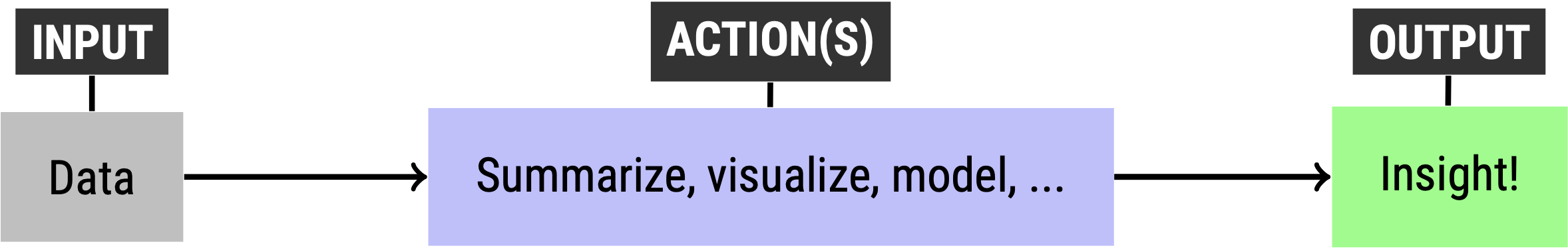
We pull this all together and restate our 1-2-3 process in R as:
And that’s it!
Income and Life Expectancy
We’re ready to do some meaningful stuff. Let’s recreate this plot:
We’ll do it in two steps:
- Summarize the data
- Visualize the data
Part 1: Summarization
gapminderSummary = gapminder %>% # 1. take the data, THEN
  group_by(continent, year) %>% # 2. organize by continent and year, THEN
  summarise( # 3. calculate:
    avgLifeExp = mean(lifeExp), # average life expectancy
    avgGdpPercap = mean(gdpPercap), # average GDP per capita
    avgPop = mean(pop)) # average population
The Gapminder Project provides GDP per capita and life expectancy around the world from 1952 to 2007:
gapmindergapminder is a data frame. We know that each column in a data frame is a vector. And we know we can calculate a statistic on a vector, like average life expectancy:
mean(gapminder$lifeExp)But that calculation pools over time and space. It’s the mean for all years (1952-2007) and all countries and continents.
What we would like to do is calculate, for example, average life expectancy within categories.
That is, average life expectancy by year, by continent, by year and by continent, and so on.
dplyr: summarize data the easy way
dplyr is a package. A package is a plug-in that makes R easier to use. dplyr is a plug-in that makes it easier to work with data frames. Moreover, dplyr is part of a suite of packages for data science known as the tidyverse. We can invoke these packages with the function library(tidyverse):
library(tidyverse)Instructions to code
Suppose we want to calculate average life expectancy, GDP per capita, and population – by year and by continent.
Let’s write down the steps, as if we were instructing a person:
- Take the data, THEN
- Organize the data by continent and year, THEN
- Calculate:
- average life expectancy
- average GDP per capita
- average population
OK. But how can we translate these to R?
Here are the translated instructions in dplyr. Run this chunk (nothing will pop out, because the output is stored in the new object gapminderSummary):
gapminderSummary = gapminder %>% # 1. take the data, THEN
  group_by(continent, year) %>% # 2. organize by continent and year, THEN
  summarise( # 3. calculate:
    avgLifeExp = mean(lifeExp), # average life expectancy
    avgGdpPercap = mean(gdpPercap), # average GDP per capita
    avgPop = mean(pop)) # average population
Let’s view the output:
gapminderSummaryThe pipe
See that %>%? That is the pipe operator. Notice how it takes the place of “THEN” in our written instructions.
%>% lets you chain together small actions on a data frame:
gapminder(take the data) THENgroupby(continent, year)(organize by continent and year) THENsummarise(...)(calculate statistics on columns)
The nice thing about the pipe operator, and dplyr in general, is that you can write code the way you would write a sentence: chaining small thoughts together one-by-one.
Part 2: Visualization
ggplot2: visualize data the easy way
ggplot2 is another package from the tidyverse. This one makes it easy to visualize data frames. Like dplyr, we can invoke it – and dplyr, and the other tidyverse packages – with
library(tidyverse)A blank canvas
The core action in ggplot2 is ggplot(). Every ggplot() follows three basic steps:
- Create a blank canvas. Every
ggplot()begins with an empty plot. You just have to feed it the data and the columns you want to visualize. Let’s put average GDP per capita on the x-axis and average life expectancy on the y-axis:
gapminderSummary %>% # take the data, THEN
ggplot(aes(x=avgGdpPercap, y=avgLifeExp)) # create empty plot- Add paint to your canvas. Layers in
ggplot2are called “geoms”. You just pick the geom that corresponds to the plot you want. If we want a scatterplot, then we add (+) the layergeom_point():
gapminderSummary %>% # take the data, THEN
  ggplot(aes(x=avgGdpPercap, y=avgLifeExp)) + # create empty plot, THEN (notice the +)
  geom_point() # add a scatterplot layer
Every new layer in a ggplot is added with +.
- Format. We can format the plot simply by adding and modifying layers:
gapminderSummary %>% # take the data, THEN
  ggplot(aes(x=avgGdpPercap, y=avgLifeExp)) + # create empty plot, THEN (notice the +)
  geom_point(aes(size = avgPop, color = continent), alpha = 0.6) + # add a scatterplot layer, with points sized by a continent's average population, colored by continent, and 60% transparency, THEN
    guides(size = FALSE) + # turn off the point size legend
  labs(title = "Live Long and Prosper", # add a title
       subtitle = "Income and Life Expectancy, 1952 to 2007", # add a subtitle
       caption = "Source: Gapminder.org | @traffordDataLab", # add a caption
       x = "GDP per capita (US Dollars)", # x-axis title
       y = "Age (Years)", # y-axis title
       color="Continent") # legend title
What should I take away from all this?
Don’t worry if you don’t understand everything about the code. The bigger picture is:
dplyrmakes it easier to manipulate data – because you can write code like you would write sentences, and;ggplot2makes it easier to visualize data, because any plot follows the same three steps.